Warm up in Regression Analysis
Warm up in Regression Analysis
Oct 29, 2018 · 8 min read

Why regression analysis?
Regression
analysis is a statistical process for estimating the relationship among
independent variables(predictors) and dependent variables(responses).
It helps to understand how the dependent variables change when any of
the independent variables is varied, while the other independent
variables are held fixed.
Some Overview….
N -> number of data points
k -> number of the weights(W) corresponding to specific parameters
model function-> Y=f(X, W)
If N<k, can’t perform regression analysis since the system is undetermined.
If N=k,
there will be a unique solution if f is linear and X are linear
independent, and it will be infinitely many or no solution if f is
nonlinear.
If N>k, there is enough information for the best-fitted model, and the degree of freedom is N-k.
Linear Regression
Linear
Regression is a statistical technique where the dependent
variable(response) is predicted from the independent
variables(predictors)
The
goal of regression analysis is using a sample from a population to
estimate the properties of the population. The coefficients in the model
are estimated the actual population parameters, so we want the
coefficient as good as possible.
Before building a linear regression model, need to ensure the assumptions:
- Linearity: the property of a mathematical relationship which can be graphically represented as a straight line.
- Homoscedasticity: the error term has mean 0 and equal finite variance at all levels of the independent variables.
- Multivariate normality: assumes that the residuals are normally distributed.
- Independence of errors: the residuals are uncorrelated with each other.
- Lack of multicollinearity: no independent variable is perfectly correlated to another independent variable.
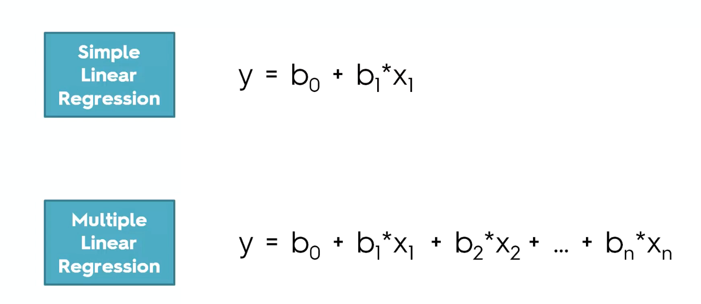
Two types of linear regression models: Simple Linear Regression, and Multiple Linear Regression.
a) If there is only one independent variable(predictor/feature), then it is a Simple Linear Regression.
b) If there are more than one independent variables(predictor/feature), then it is a Multiple Linear Regression.
For the Categorical variable, we
need to create dummy variables which are converting the information
from the categorical variable. (Caution: we always need to omit one
dummy variable because since n-1 dummy variables are known, then we will
know the last one!)
Polynomial Regression
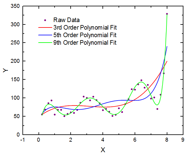
The polynomial regression reveals the relationship between the independent variable and the dependent variable as an nth degree polynomial
in the independent variables. Normally, the polynomial regression
function is a non-linear function, and it can be fitted with discrete or
continuous features. It is a way to prevent the underfitting problem from linear regression since it increases the model complexity.
Logistic regression (linear classifier for classification)
Logistic
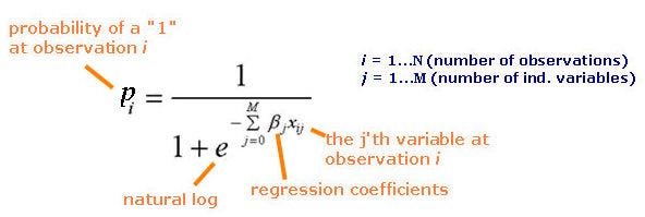
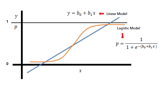
Regression is using the logistic model to predict the binary outcomes
from a linear combination of the predictors. Unlike Linear regression to
output a set of numeric values, Logistic Regression will output the
probability that given input belongs to a specific class.
Logistic regression is conducted when the dependent variable is binary, which can be discrete or continuous. In logistic regression, the response (dependent variable) has a finite number of possible outcomes.
Adding independent variables will always increase the variance of the model toward overfitting.
Before building a logistic regression model, need to ensure the assumptions:
- The dependent variable(response ) should be binary in nature.
- There is no outlier in the data.
- Lack of multicollinearity: no independent variable is perfectly correlated to another independent variable.
- Need to make sure the input data can be separated into two ‘regions’ with a straight perceptron boundary.
Why the threshold of the logistic regression model is 0.5?
Since
the optimization technique to find the best sigmoid curve, we apply the
MLE to estimate the parameters. The criterion is we need to try the
best to make every sample labeled in ‘1’ will have a logistic function
result close to 1, same logic for label ‘0’.
Decision Tree Regression
Tree-based
model: it breaks down the data into smaller and smaller subsets while
at the same time an associated decision tree is incrementally developed.
The final result is a tree with decision nodes and leaf nodes.
If the target variable is continuous numeric values with infinite possible outcomes, then the decision tree is called regression trees.
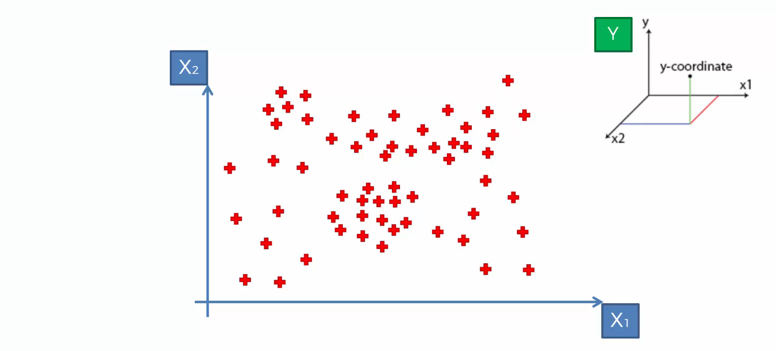
Mathematical Formula:

The logic of decision tree is recursively splitting the tree into binary sub-trees:
- In each split, consider all predictors as the possible split attributes. For each predictor, the data is split into several split points, and then select the best split point for the specific predictor(independent variable) by evaluating the Sum of Square error(SSE)(lowest is the best). Repeat choosing the best split point for every predictor, then choosing the final best split point by evaluating the Sum of Square Error of all ‘best’ split points of all predictors at the same level.
- Repeat step 1 split the tree into sub-tree recursively, until we meet some stop criterion below.
Stop Criterion:
Since the decision tree can be split until there is only one element in
each node. Normally, such trees are quite complex and leading to
overfitting with high model variance. Therefore, it is a need to set a
stop criterion.
- we can set a threshold as the minimum number of input in each leaf, the tree stops splitting while parent-node reaches the threshold.
- we can set a threshold as the maximum depth the tree can go, the tree stops splitting while it reaches the specific number of depth in the tree.
- we can set a threshold as the target sum square error, the tree stops splitting while there is a large decrease more than the threshold, compared to its parent node. However, according to the greedy algorithm, it is possible to find good split after bad split. (not robust)
- Predictor values for all records are identical.
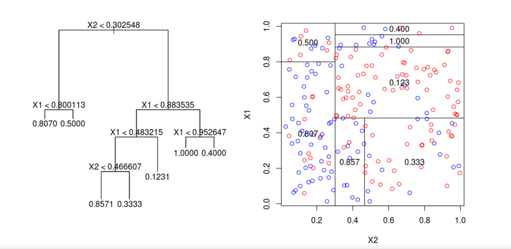
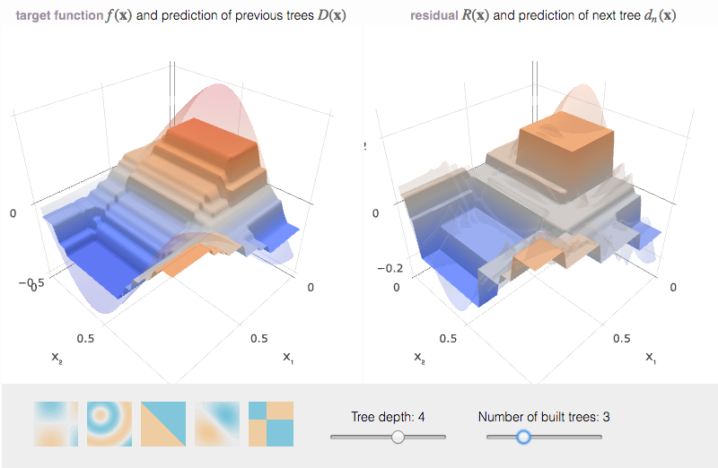
Worthy to mention: the ‘region’ of the decision tree in regression must satisfy the following criterions:
a) Disjoint (no parallel split perceptron into another split perceptron)
b) cover the whole space (split perceptron has to split the whole involved space)
Advantages:
a. Simple to understand and interpret.
b. Requires little data preparation — normalization.
c. Mirrors human decision making more closely than other approaches.
Disadvantages:
a. a small change in training data will cause a large change in the decision tree.
b. practical decision-tree learning algorithms are based on heuristics such as the greedy algorithm
where locally optimal decisions are made at each node. Such algorithms
cannot guarantee to return the globally optimal decision tree.
Random Forest Regression
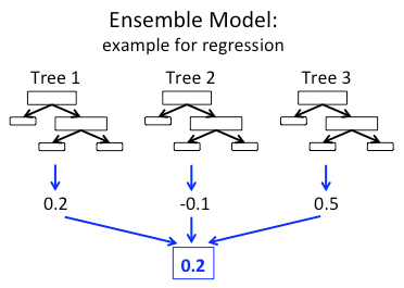
The random forest model is operated by constructing a multitude of decision trees on many bootstrap samples(re-sample with replacement) via bagging method at training time and make the final prediction with the average of the prediction across the trees.
Advantages:
a)
Prevent overfitting: by averaging prediction from trees, significantly
reduce the risk of overfitting, therefore more accurate.
b) Run efficiently on large databases, and it can handle thousands of input variables without variable deletion.
Support Vector Regression (SVR)
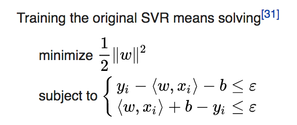
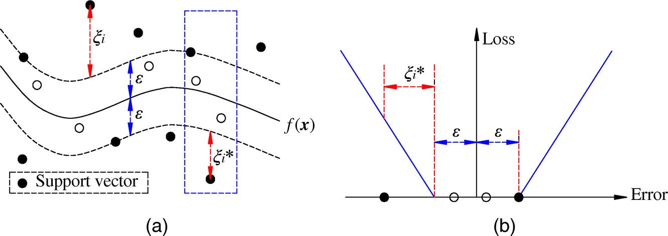
SVR is a type of support vector machine that supports linear and nonlinear regression.
It
produces by Support Vector Machine(SVM) depends only on a subset of the
training data, because the cost function for building the model ignores
any training data close to the model prediction within the absolute
difference of epsilon.
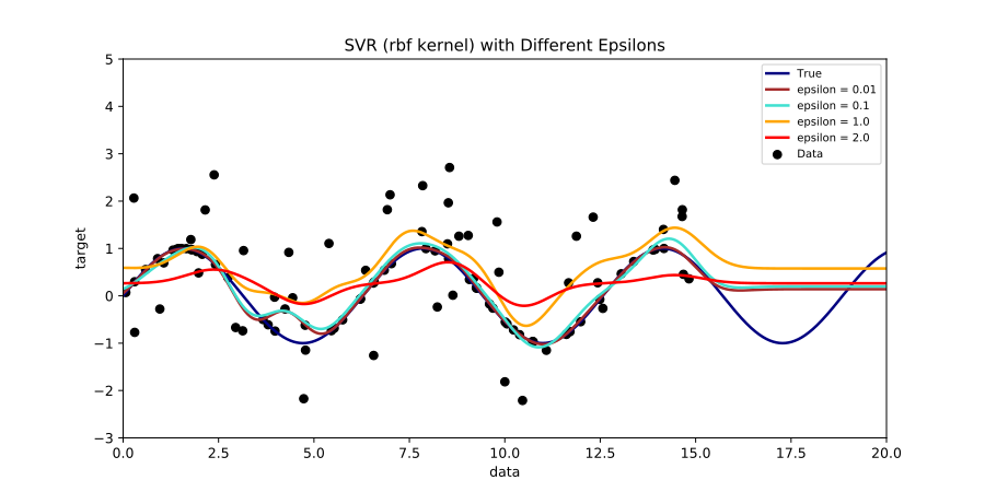
With different thresholds ε, the model is flatter. As ε increases, the prediction becomes less sensitive to errors.
Optimization Techniques:
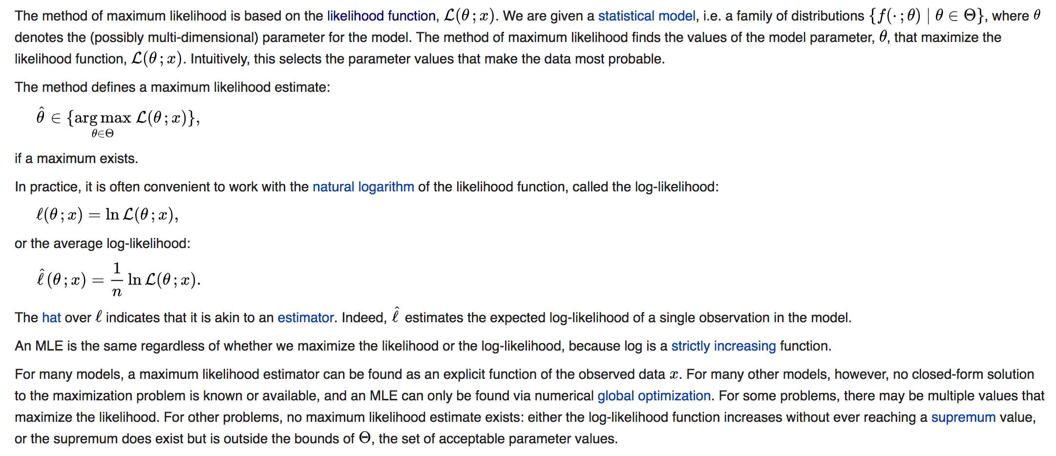
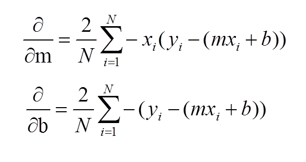
- Maximum Likelihood Estimation (More details will publish in latest post):
2. Least Square Estimation:

Regression Model Evaluation Metrics…..!
- RSME (root mean square error): it represents the sample standard deviation of the difference between predicted value and observed values, and it is also known as residual. The formula is:

2. MAE (mean absolute error):
it represents the absolute difference between predicted values and
actual values, and it also means all individual differences are weighted
equally. The formula is:

RMSE v.s. MAE:
Similarities: They both range from 0 to 1, and the lower value indicates the better result.
Differences:
a.
MAE directly take the average of the offset, RMSE penalizes the higher
difference between the actual and predicted values more than MAE.
b. RMSE ≥ MAE, and they only equal to each other when all differences between the actual and predicted values are zero.
c.
RMSE is more practical because the loss function defined in RMSE is
smoothly differentiable and make it easier to perform in mathematical
operations.
d. RMSE is easier to solve, but MAE is more robust to outliers.
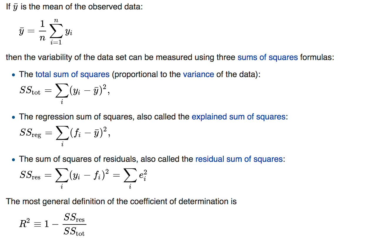
3. R square (R2):
it represents the proportion of the variance for a dependent variable
explained by the independent variables. In other words, it measures how
well the observed outcomes are replicated by the model. The formula is:

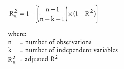
4. Adjusted R square:
it measures how well the independent variables fit a curve or line as
well as R2 but adjust for the number of independent variables in a
model. The formula is:
R2 v.s. Adjusted R2:
a.
R2 increases or stay the same with the addition of more independent
variables, even they don’t have relationships with the dependent
variables.
b.
Adjusted R2 provides an adjustment to R2 statistic such as the
independent variable has a strong correlation to the dependent variable
will increase Adjusted R2, but decrease while the adding variable
doesn’t have a strong correlation with dependent variables.
Pros and Cons of Regression Evaluation Metric:
- RMSE is the better choice if we only care about model accuracy.
- Any metric such like MAE which doesn’t take the square of the difference is more robust to outliers.
- Any square of error term metric should be more useful when large errors are particularly undesirable.


Comentários
Postar um comentário